Help: THERMOS Heat Demand Model

The space heat demand model is an set of regression models, one of which is selected depending on which facts are known about the building. The regression models are trained on data from Copenhagen, where we had access to annual per-building metered demand, together with LIDAR and building polygons. From the LIDAR and building polygons we derived several predictors, used as inputs to building the regression models.

We trained four models, to cover four conditions that can happen:

1. A support vector machine (SVM) using all of the known predictors
2. A linear regression (LM) using all of the known predictors
3. A SVM using only those predictors available without a building height estimate
4. A similar LM

Each model is in fact trained to predict the ratio of space heat demand to square-root heating degree days.

This is used together with a rule of thumb from this project that, all things being equal, heat demand between two locations varies with the ratio of the square root of heating degree days in those locations to allow the model to be used in different places.

When making an estimate for a building, one of these models is selected thus:

ensemble.pdf

The application takes building height from a number of places:

1. If the building dataset directly includes a building height field, that is used
2. Otherwise if LIDAR is available the building height is estimated by finding ground level as the bottom decile of height in a buffer around the building and then subtracting that from the mean LIDAR height within the building's footprint.
3. Otherwise if the building dataset includes a number of storeys, height is estimated as the number of storeys multiplied by 3m (assuming an external storey height of 3m)

We trained the regression models using the following features as inputs, using a feature selection process to find the subset which gave best performance without overfitting. The columns indicate which features are used by which models. Many of the features are correlated with each other, which explains why only a few have ended up in the model.

Feature	2D	3D
Footprint	Y
Perimeter	Y	Y
Shared perimeter (%)	Y
Shared perimeter (m)	Y
Is residential	Y
Perimeter / footprint
Height		Y
Volume (footprint x height)		Y
Surface area / volume		Y
External wall area		Y
Surface area
1/(Surface / volume)2
Floor area
External surface area
External SA / volume
Wall area

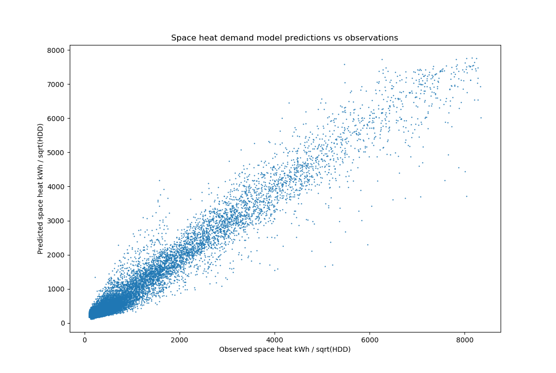
For the 3D SVM, measured on the training data, the model's root mean squared error (RMSE) was 195 kWh / (deg day)^0.5. This corresponds to a mean percentage error of 10.7%. When cross-validation was performed, the average RMSE across the five cross-validation sets was 205 kWh / (deg day)^0.5, and the mean percentage error was 10.5%.

The linear and 2D models perform less well, as might be expected.

In addition, we validated the 3D demand model by testing it on unseen data, using a set of buildings from 16 locations across the UK. While it was possible for us to produce the geometric features for individual buildings, we did not have access to building-level energy consumption data.

Instead, energy consumption totals were available for regions called middle super output layers (MSOAs). An MSOA is an aggregated UK census geography containing around 4,000 households. The set of MSOAs comprised eight pairs, one urban and one rural, with each pair lying close to an airport whose weather station data provided the HDD.

The MSOA consumption statistics give metered fuel totals. From these totals we estimated the total heat demand by the following formulae:

• for domestic buildings: Q_heat = 0.85 × Q_gas + 0.55 × Q_{economy 7} + 0.1 × Q_elec
• for non-domestic buildings: Q_heat = 0.85 × Q_gas + 0.1 × Q_elec

Here, the factor 0.85 is the assumed average boiler efficiency, the factor 0.55 is the assumed fraction of off-peak electricity used for heating, and the factor 0.1 is the assumed fraction of on-peak electricity used for heating.

We then compared the sum of model predictions with the sum of the estimates derived from MSOA-level metered consumption:

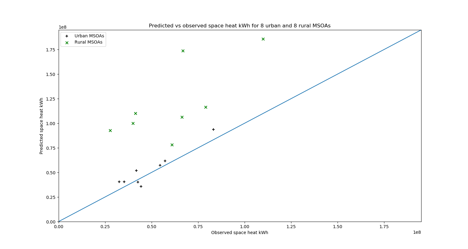
While there is good agreement for urban MSOAs, the results for rural areas are less positive, with the total space heat being over-predicted in every case. The poor performance in rural areas is perhaps not surprising, since the model was trained entirely on data from urban areas (Copenhagen and Aalborg).

Another possible explanation for the over-prediction is that large unheated buildings, such as agricultural structures, are more common in rural areas - in the absence of data flagging this, such buildings will be assigned a demand value by the predictive model, contributing to an overestimation of demand at MSOA level.

Finally, in rural areas in the UK it is not unusual for heat demand to be met using unmetered fuels such as LPG, oil and biomass. These data are not accounted for in the MSOA-level consumption totals, which hence are likely to systematically under-represent heating demand in rural areas.

The SVM models use a radial basis kernel, which has the effect of clamping predictions for points that lie outside the training set to the edges of the training set. This means that the SVM models cannot 'extrapolate' outside the range of values seen in the training set. To allow extrapolation, we fall back to the linear models if one of the predictors for a building is much outside the range seen during training.

Since the square-root degree days transfer does not apply for hot water demand, we estimate that separately using SAP 2012, the UK Government's Standard Assessment Procedure for Energy Rating of Dwellings (https://www.bre.co.uk/filelibrary/SAP/2012/SAP-2012_9-92.pdf page 184, Section 4).

In training we subtract the SAP prediction from the measured value, and when predicting we add it on.