1. Outputs from the network model
Two outputs from THERMOS' network model are:
A list of buildings that are connected to the heat network.
Each building has a peak demand (kW" and an annual demand (kWh/yr).
- A peak demand and annual demand for the network's supply point
2. Inputs to the supply model
These demands are not detailed enough for supply-side modelling, which depends on prices that vary on an hourly or half-hourly basis across the year. More detail of this is given below, but for now the important point is that the supply model's decisions are over a large number of time intervals representing a typical operating year.
For example, if modelling the year as 5 representative "day types", each having 48 half-hourly intervals, there are 240 half-houly heat demand intervals that need to be modelled. However, we only have two facts (peak and average demand) about heat at the supply point, and at each building.
Because of this, THERMOS needs a way to convert these summary statistics into a load profile for the supply location which says how much heat is required in each modelled interval.
3. Creating a load profile
This is done in two stages:
First, for each building, we contruct a load profile for the building by deforming a profile shape for that building so that it has the right peak demand and annual demand.
The profile shape itself is a user input describing a relative heat demand in interval.
A profile shape like this can be adjusted easily to have a given peak value - we just have to divide each interval's value by the maximum in any interval (effectively normalising the profile shape), and then multiply by the desired peak. However, this operation will probably not give the desired annual demand; in truth there are an unlimited number of possible profiles that fit a given annual demand and peak demand, but we need some way to construct one that looks realistic.
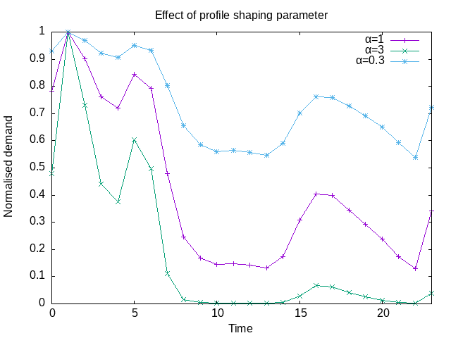
In THERMOS this is done by compressing or stretching the normalised profile shape, so that it has the desired annual demand once it's multiplied by the desired peak. The compression or stretch is the same for each interval, and is determined by a "flattening" parameter α: in a given interval, if the normalized value is \(x\), the deformed value is \(x^α\).
Since the values in the normalized shape range from 0 to 1, no choice of α can move any of the intervals outside that range. An α of 1 makes no change to the shape; an α of 2 makes the shape "peakier" (since all of the sub-peak intervals are squared, and being less than 1 this reduces them); an α of 0.5 makes the shape flatter (each interval is square-rooted). In the limit, an α of infinity makes every point except the peak have value 0, and an alpha of 1 makes every point have value 1.
The required value of α is determined numerically, allowing the construction of a per-building load profile which has a peak & average demand that reflect the values seen by the network model.
Next, for the supply, we sum all the load profiles for the buildings, and then repeat the profile deformation process so that the resulting peak and average demand equal the values predicted by the network model for the supply point.
This is not just the sum of all the building profiles because of the load diversity effect, which flattens the peak a bit.
This final reshaped load profile gives a heat demand on the supply for each interval, in each representative day being modelled.