1. Top bar and sidebar

Figure 1: THERMOS top bar, from left to right: sidebar button, problem name, save button and optimise button.
The top bar is always visible.
- On the left is the THERMOS logo. Click this to open the sidebar to change pages.
- In the middle is the problem name. The latest save for each name is shown in the project page (although you can access earlier versions).
- To "Save As", change the name and press save
- The Save button. Can't hurt to click this
The Optimise button, to run the model.
When you click this it will show three options:
- Network : run the network model only
Supply : run the supply model only, using the last network model solution.
There must be a network model solution for this to do anything.
- Both : run the network model, and then run the supply model using the results from the network model.
2. Map view
2.1. Keyboard shortcuts
There are a few single-key shortcuts in the map view:
| Key | Action |
|---|---|
| c | Cycle the constraint status of the selection |
| (press repeatedly to cycle through the options) | |
| e | Show the candidate editor for the selection |
| s | Show the supply editor for the selected buildings |
| g | Select all buildings in same groups as any selected buildings |
| G | Make all the selected buildings belong to a single group |
| U | Remove all the selected buildings from any group |
| z | Zoom to show the selection, or the whole problem if no selection |
| a | Select every un-forbidden candidate |
| A | Flip the selection (select unselected, and deselect selected) |
2.2. Resizing and toggling panels
The map view is split into three regions: a map, the selection info panel on the right, and the network candidates panel at the bottom.
You can change the size of the panels by clicking and dragging on the grey border between them.
You can quickly hide or show a panel by clicking on the little arrow button in the middle of the grey border:  .
.
2.3. Selecting things
The main purpose of the map view is to select candidates (these are buildings or pipe routes), and then to manipulate or investigate them. The selection refers to the set of candidates which are selected at any time.
The selection is ephemeral and only one selection exists at a time, much like a selection in a spreadsheet program. There is no quick way to save or recall a selection, so if you want to do something very complicated it is best to do it a bit at a time.
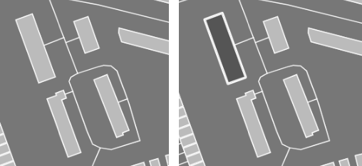
Figure 2: Difference in appearance due to selection. On the left nothing is selected, on the right the top-left building is selected.
You can see on the map whether something is selected by the style with which it is drawn. Selected buildings are drawn with a darker colour, and selected paths or buildings are drawn with a thicker line.
Clicking on a thing with the mouse is the simplest way to select it. This will also deselect whatever is currently selected. Clicking in an empty space will therefore clear the selection.
If you want to select several things by clicking on them, you can use modifier keys to change what happens. Holding down a modifier key while clicking will control how the selection is affected:
- Shift+click
- Holding the Shift key while clicking will add whatever is clicked to the selection, without unselecting what was selected before.
- Control+click
- Holding the Control key while clicking will invert membership of the selection, without changing the rest of the selection. For example if you Control-click something that is in the selection, that thing will be deselected. If you control click something which isn't selected, it will be added to the selection.
There are other ways to control the selection, which we will come onto in:
2.4. Map controls
Around the edge of the map are some control buttons:

Figure 3: Map controls on the left. From top to bottom: Zoom In, Zoom Out, Select Polygon, Select Rectangle, Hide/show forbidden, Zoom to network, Add Connector and Add Building buttons.
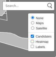
Figure 4: Map controls on the right. The search box searches Nominatim for places (it does not unfortunately search THERMOS map data specifically). The box below controls what is displayed on the map.
2.4.1. Moving the map
To change the area displayed on the map you can:
- Pan by clicking and dragging with the mouse
- Zoom in and out by
- clicking the buttons in the top left
- scrolling your mouse scroll-wheel if you have one
- pressing the - or + keys on the keyboard
- holding Shift and then dragging a rectangle on the map
- Search for a location using the search box in the top right. This searches an index of place names, rather than information within the map
2.4.2. Area selection
You can select several buildings in an area with the area selection buttons, below the zoom buttons.
The first one (with a pentagon on it) lets you select using an irregular polygon. Click this to start selecting an area, and then click at points on the map to make a shape.
When you click on the last point, every candidate intersecting with the shape will be selected.
The second button (with a square on it) lets you select by drawing a rectangle. Click the button, then click the map at the top left and bottom right corners of the rectangle you want to select.
2.4.3. Hide/show forbidden
Below the area selection buttons is the Hide/show forbidden button, illustrated by a grid of four squares. This button will toggle the map between displaying forbidden candidates or not - turning off forbidden candidates may make it easier to focus on your problem once you have decided what is in it.
2.4.4. Zoom to network / selection
This button has a crosshair on it - clicking it will center and zoom the map to the selection, or all non-forbidden candidates if the selection is empty. You can also press the z key for this.
2.4.5. Draw connector
Next is the connector drawing tool ( ).
).
Clicking this puts the map into a special mode where you can draw new connecting lines. To add a connecting line:
- Click the connector drawing tool button
Click on the candidate where you want the line to start - for example on a building whose connector is in the wrong place.
The starting candidate will be highlighted with a thick dotted line
Click on any intermediate points on the map you want the connector to go via.
As you click the connector will be shown as a dotted line:
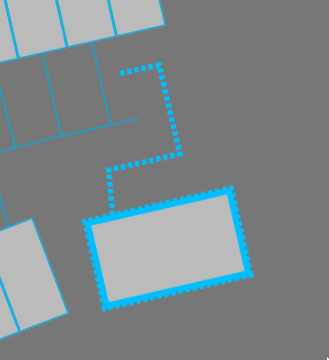
Figure 5: Halfway through drawing a connector
To finish the connector click where you want it to connect to. Generally you will want to go from a building to a path, a path to a building, or a path to a path.
Connecting two buildings will have no effect unless one is a supply point.
To cancel drawing a connector, click the connector tool button rather than finishing the line.
2.4.6. Draw building
Below the connector drawing button is the button to add a new building. To use it, click the button, and then click where you want the building to go.
The new building will always be rendered as a circle, and you will probably immediately want to edit it with the e key or s key since new buildings have no demand or supply information set on them.
2.4.7. Map display controls
On the right you can control what is shown on the map.
There are two sets of controls:
- Controls for the basemap, which is displayed underneath the candidates. This is a single exclusive choice between:
- None
- This displays a blank grey background, which helps the candidates stand out
- Maps
- This displays a black & white cartographic map called Stamen Toner, which uses OpenStreetMap data
- Satellite
- This displays satellite or aerial imagery from ESRI
- Controls for what is on top of the basemap, which is a multiple choice of:
- Candidates
the network candidates (buildings and paths).
When zoomed out a lot, this will show only buildings and paths from any solution network.
- Heatmap
- an indicative heat density layer drawn on top of the candidates
- Labels
- a layer showing street names (also part of Stamen Toner).
2.4.8. Map view / solution display
At the bottom of the map is a control which switches the map display between two modes:

Figure 6: Map view control, set to solution display. You can use the Map legend button on the right to get a reminder of what colours on the map indicate.
Clicking either of the two buttons on the left of this section change how colour is used in the map.
When Constraints is selected, the colours in the map show information about the problem:
- Blue elements are optional for inclusion in the network, if they improve the solution
- Red elements are required to be included in the network, whether or not this improves the solution
- Supply sites are coloured in orange
- Everything else is forbidden
However when there is a solution and Solution is selected, the map changes to show information about that solution. In this case:
- Red elements are in the network
- Yellow elements are peripheral pipes, reachable by the network but not useful
- Magenta elements are not reachable from any supply location, so could never be connected
- Green elements have alternative heating systems selected (when the objective allows this)
- Supplies that have been built are coloured in orange
- Everything else is drawn in grey
To the right of these you can also toggle whether to show pipe sizes.
This will scale the thickness of line used according to pipe diameter, making bigger pipes draw with thicker lines. This can help you see the network structure on the map.
2.5. Selection info panel
The selection info panel is the region on the right hand side of the map view. Typically it will look something like this:
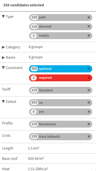
Figure 7: Example of the selection info panel. The Category and Name rows are elided.
This panel tells you all about the currently selected candidates. At the top, you can see how many candidates are selected.
Below that are a number of rows - which rows are visible will depend on what is selected. Each row has a label on the left, and information on the right.
These rows typically display two types of information: categorical values or numeric ones. Categories are displayed as a series of chips, where each chip indicates how many of the selected candidates fall into that category.
Sometimes category rows are elided, to keep the panel short. For example in the image above Category and Name are elided. Clicking on the triangular arrow by the label will show or hide the different categories.
Numerical values are aggregated up in a sensible way, depending on what is being displayed - some will be summed up, others averaged and so on. Most numerical values will show you some more detail (min, max, etc) if you hover the mouse over the value - this is usually indicated by a little superscript blue letter i.
2.5.1. Narrowing the selection by category
All the categorical rows in the selection info panel can be used to narrow down the selection. This is a useful way to quickly find particular buildings or roads.

Figure 8: The category row for candidate type. This shows that in the selection, 239 candidates are paths, 118 are demand buildings, and 1 is a supply building. Note how each chip has a little cross on the right.
- Deselecting a category
- To deselect all candidates in a category click the cross on the right of the chip. For example in the picture above, you could deselect all paths by clicking the × next to paths.
- Selecting a single category
To select only candidates in a category, click the name on the chip. For example, above you could find the supply by clicking supply. This would be like clicking × on path and demand.
After this you might want to press z to find the selected thing on the map.
2.5.2. Type
The type field will always show one of three values: path, demand or supply, which are self-explanatory. A detail is that supply and demand are exclusive here, although they are not exclusive for the model. If a building is both a demand and a supply, the type field will say supply
2.5.3. Constraint
The constraint field will always show one of three values: forbidden, optional and required. These are colour-coded to match the display on the map, when the map is set to show constraints. See Constraint status above for more information about what these mean.
2.5.4. Tariff
The tariff field says what tariff a building is on. This affects how much revenue the network would receive if it were to sell heat to the building.
For more on tariffs see Tariffs above under concepts. To define tariffs see the section below about Tariff definitions.
2.5.5. Edited
If you have edited something about a building in this problem, this will say yes. Otherwise no. Note that edits live within a problem, so the underlying map will not be affected - new problems in the same map will start from the original status in the map.
2.5.6. Profile
A building's profile is part of its connection to the supply model - for more detail see the section on how the supply model is joined to the network model.
2.5.7. Civils
A path's Civils affect the cost for putting in a pipe. For more about civils see Civil costs in the concepts section above.
2.5.8. Length
A path's length in metres. If multiple paths are selected, gives the total length.
2.5.9. Base cost
Depending on what is selected, gives an indicative cost. For buildings, this is the connection cost. For paths it is the minimum pipe cost on that path.
2.5.10. Heat (or cold) demand
This shows the summed annual heat demand for selected buildings. This is without any insulation applied.
2.5.11. Heat (or cold) peak
This shows the summed peak heat demand for selected buildings. This does not account for diversity, nor the installation of individual systems which may smooth the peak, so it may be lower than the peak output from network supplies or individual systems.
2.5.12. Insulated demand
When displayed, this shows the total heat demand that the selected buildings required in the solution. This can be lower than the heat demand row, because the model may install insulation.
2.5.13. System peak
When displayed, this shows the total peak demand that the selected buildings required in the solution. This can be lower than the peak row, if the buildings were allocated individual systems for which the tank factor is set.
2.5.14. Lin. density
Shows the linear heat density of the selected candidates. This is calculated as the total annual heat demand of the candidates (without insulation) divided by the total length of any selected paths.
2.5.15. In solution
When a problem has been solved this row will be displayed. It can take a few values:
- network
- the candidate is part of a heat network
- no
the candidate is not part of a network, nor has it been given an individual system.
For buildings, this can happen if (a) the objective is network NPV or (b) the objective is whole-system NPV but no individual system is on offer because (i) individual systems are not enabled, or (ii) they are enabled but this building has no counterfactual or alternative heating choices set.
For paths this just means they are not in a network
- impossible
- this means that the candidate was never considered for networking, because it is not reachable by any route from any supply location.
- peripheral
- this is only shown for paths; it means that a path is reachable from a supply, but it does not connect that supply to any demands, so was ignored.
- other options
- if a building has been given an individual system, the name of that system will be shown here.
2.5.16. Losses
Shown for paths, this is the summed annual heat loss calculated for these paths, given in total and per-metre.
2.5.17. Coincidence
Shown for paths, this is the biggest diversity effect that has been applied to any of the selected paths. This shows how much smaller the pipe's maximum capacity is than the sum of the peak demands it is serving.
2.5.18. Capacity
Shown for paths and supply points, this is the largest capacity in kW required across the selected candidates in the model's solution.
2.5.19. Principal / PV Capex / Σ Capex
This row has a menu on the left to change what is shown. It is shown for anything that the model has spent money on in a solution.
This shows the capital cost spent on the selected items. For paths, this is the cost of pipes. For buildings, this the capital cost part of connection cost, plant cost, individual system cost and insulation cost.
The different choices are:
- Principal
- This is the upfront capital cost, without any cost of replacement or financing
- PV Capex
- This is the present value of the capital cost, replacement costs, and any finance costs
- Σ Capex
- This is the undiscounted version of PV capex, so all capital costs and finance costs
2.5.20. Revenue
Shown for buildings, this is the annual revenue that building provides to the network operator
2.5.21. Market rate
Shown for buildings in a network on the market tariff, this is the unit rate the system has decided to offer them.
2.5.22. Other user-defined fields
Candidates may have arbitrary other fields added to them, either when uploading GIS data for a map, or within a problem by using the candidate editor (explained below).
If these fields are categorical they will be displayed as chips (like built-in categorical information); if numeric as numbers, where the sum will be displayed across the selection.
2.6. Network candidates panel
The network candidates panel is at the bottom of the screen.
It is a table, listing all of the candidates whose status is not forbidden.
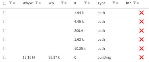
Figure 9: An example of the network candidates panel
At the top are column headers; below that each row corresponds to a candidate.
2.6.1. Selection column
In the header and in each row of the panel is a checkbox (little square).
Clicking the checkbox in the header row will select or unselect all candidates (this is like pressing a or a A). Clicking the checkbox on a given row will select or deselect that row. The selection is reflected on the map and in the selection info panel.
2.6.2. Sorting and filtering
The selection info panel can be sorted by any of its columns, by clicking on the header label. One of the small up/down arrows will be highlighted blue to show what the sort order is.
The panel can also be filtered by any of the columns, by clicking the small icon that looks like a funnel ( ). This will show a filter dialog, that lets you restrict which rows are displayed.
Candidates whose rows have been filtered out are made slightly transparent on the map:
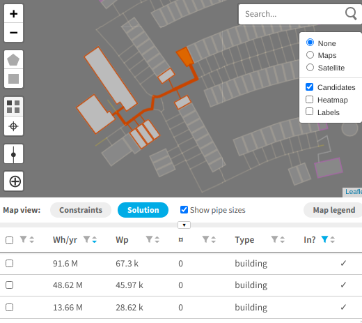
Figure 10: Filtered selection info panel. Note that the In? column is filtered (its filter icon is blue), and the map is highlighting those elements which are on a network.
2.7. Editing candidates
When you have some candidates selected you can edit what the model knows about them by pressing the e key (or by right clicking on them).
This will bring up a box with several sections which let you change information about the selected candidates.
2.7.1. Editing demands
Shown only when the selection includes some buildings.
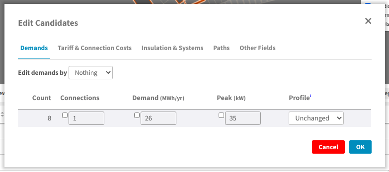
Figure 11: Editing all selected demands
The first thing to notice here is the menu saying Edit demands by: Nothing.
When you have several candidates selected, you might want to edit them differently depending on information about them.
For example, here is the same edit window with the menu changed to the Category field:
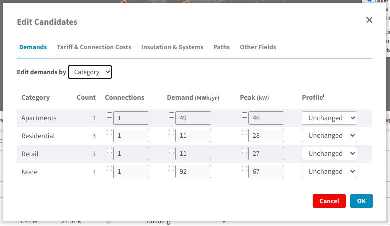
Figure 12: Editing demands by category
Now the single row representing everything is split into four rows for the four selected categories.
Changes to the Retail row will affect the single selected apartment, whereas changes to the Residential row will affect the three selected Residential buildings.
In each row you can see four columns that you can edit. The numeric columns have a checkbox next to them - to edit a cell, check the checkbox. The profile column has a special Unchanged value to leave the profile setting alone.
- Connections
- changes the connection count for each of the selected buildings. This affects diversity calculations.
- Demand
- sets the annual demand for each selected buildings
- Peak
- sets the peak demand for each selected building
- Profile
- sets the profile class for each selected building. This is used to produce a load profile for the supply model.
2.7.2. Editing tariff & connection costs
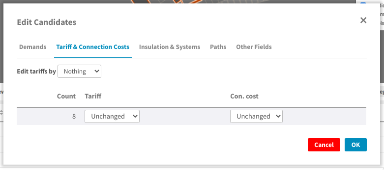
Figure 13: Editing tariffs
This page lets you set the tariff and connection cost applied to the selected buildings
2.7.3. Editing insulation & systems
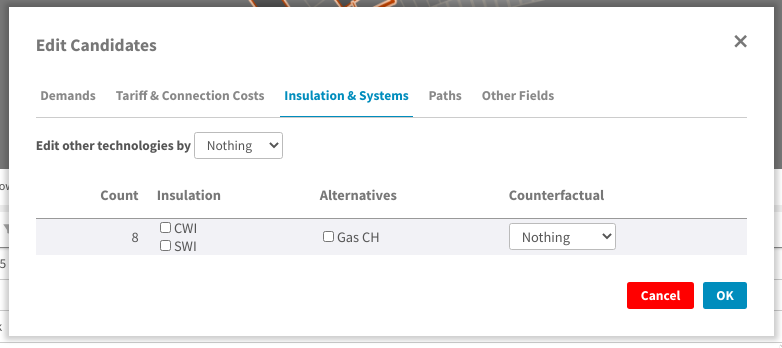
Figure 14: Editing insulation and systems
This page lets you select the other technologies offered to the building, when in whole-system optimisation mode.
- Insulation
- Selecting or unselecting these checkboxes will make the selected buildings eligible or ineligible for these types of insulation
- Alternatives
- Selected checkboxes here determine which alternatives to a networked heating system are offered
- Counterfacetual
- This lets you tell the model what heating system a building already has, making it available as a "do-nothing" option with no upfront capital cost.
2.7.4. Editing paths
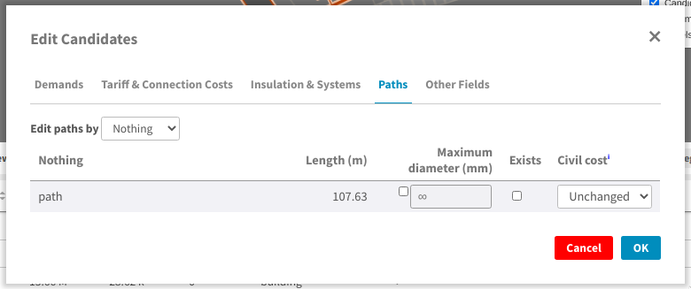
Figure 15: Editing paths
For paths you can set:
- Maximum diameter
- This will prevent the model from installing a pipe larger than this diameter
- Exists
- If checked, the path already has a pipe in it, so its initial capital cost will be zero
- Civil cost
- Controls the civil cost category for the path, which affects the cost of installing a pipe
2.7.5. Editing other fields
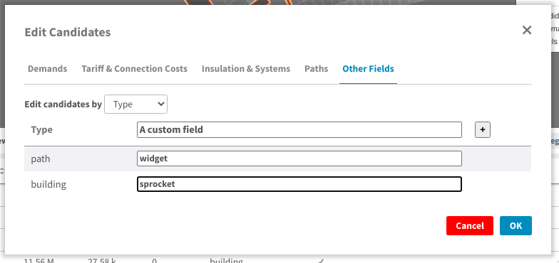
Figure 16: Editing other fields
Other fields have no effect on the model itself, but are visible in the selection info panel.
You can use them to mark particular buildings to keep track of them, and they can be loaded in from external GIS data when creating a new map.
To set a custom field:
- Click the + button in the header. This will add a new column.
Type the field name in the cell that appears in the header for the new column.
A dropdown menu will let you select existing fields for the selection, or you can type an entirely new name to create a new field.
- Type the values you want into the cells underneath.
2.8. Adding supplies & changing supply parameters
Any building can be made into a supply point, and to model a heat network you'll have to make at least one - THERMOS doesn't know about where any supply locations are unless you tell it. If you want to consider a supply that is not in an existing building, you can use the draw building tool to make a new building.
To make a building into a supply, select it and press the s key (or right click and choose from the menu).
This will show the supply parameters box:
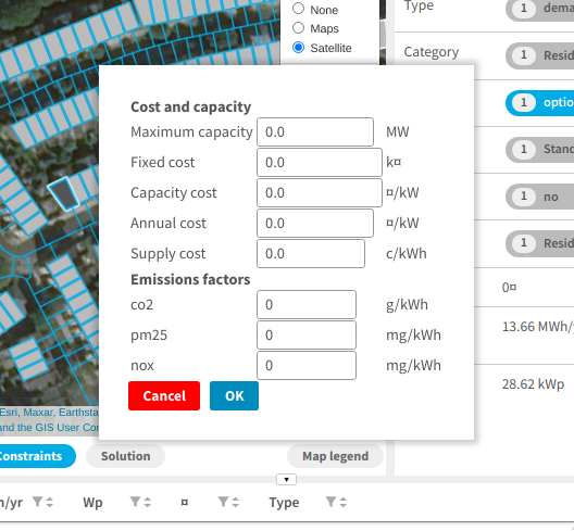
Figure 17: A supply parameters window; to make the selected building(s) into supply points, enter a nonzero capacity.
The parameters in this box determine the cost and size of the supply for the network model
- Maximum capacity
- This is the maximum amount of diversified peak load a supply built here could provide. The model may build a smaller supply if that will suit, but never a larger one.
- Fixed cost
- If any supply is built, no matter its size, this fixed capital cost will be incurred. See above for information about the treatment of capital costs.
- Capacity cost
- This is a variable capital cost per unit of diversified peak capacity that is built, reflecting the increased cost of building a bigger plant.
- Annual cost
- This is an annual operating cost per kW diversified peak capacity.
- Supply cost
This is the price of producing a unit of heat at the supply. This is multiplied with the system's output and losses each year to determine the cost of heat that was produced.
If you have a fuel cost A and a nominal efficiency B this should probably be A/B
- Emissions factors
- These determine the emissions the supply is responsible for, per unit of heat output. Similarly to fuel cost, you will probably need to incorporate an efficiency into these values.
2.9. Grouping buildings
Sometimes you may want the model to connect a set of buildings all together or not at all - this could represent a development that has several buildings in it, for example. It can also help simplify the optimisation problem, as the optimiser has fewer decisions to make.
Each building can belong to a single group of buildings - the optimiser will treat that group as a single decision.
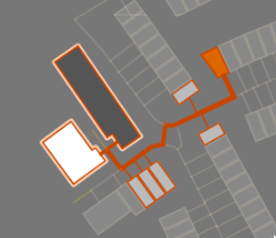
Figure 18: The centre building is selected. The leftmost building is in the same group, which is why it is filled in white. The optimiser can choose either to connect both these two or neither, but nothing in between.
To create a group, select a set of buildings and press Shift+G. The selected buildings will be made into a group.
If any of them were previously in other groups, they will be taken out from these groups.
When you have some buildings selected you can see any other buildings which are in a group with any of them coloured in white. You can select everything in the same group by pressing g.
2.10. Deleting things from the map
Sometimes you may want to delete something from the map; for the optimiser this is no different than marking it forbidden, but it can make things easier to look at. You can do this by right-clicking on the item you want to delete, and choosing Delete.
3. Objective
See also the section above.
The objective setttings page lets you control things about the model's objective function, and how the optimiser behaves.
3.1. Choice of objective
The model has two main objectives, selectable on the objective page in the sidebar:
Maximise network NPV
In this mode, the goal is to choose which demands to connect to the network so as to maximize the NPV for the network operator. This is the sum of the revenues from demands minus the sum of costs for the network.
The impact of non-network factors (individual systems, insulation, and emissions costs) can be accounted for using the market tariff, which chooses a price to beat the best non-network system.
Maximise whole-system NPV
In this mode, the goal is to choose how to supply heat to the buildings in the problem (or abate demand) at the minimum overall cost. The internal transfer of money between buildings and network operator is not considered, so there are no network revenues and tariffs have no effect.
Under this you can control whether or not to
- Offer insulation measures
- Offer other heating systems
These choices are not relevant when maximizing network NPV, because they can never improve the network operator's NPV so would never be chosen.
3.2. Accounting period
Future costs and benefits are combined using geometric discounting. The accounting period controls let you set the number of years into the future to consider, and how much to discount a cost by for each year from the start of the simulation.
3.3. Capital costs
Capital costs have two types of special treatment:
- Annualizing
- capital costs can be annualized, which means converting them into a fixed repayment loan
- Recurrence
- capital costs can recur, which means that the equipment they represent needs replacing every so often, so the original capital cost is incurred again after this time.
The capital costs section lets you control for each part of a solution:
- Whether it should be annualized and whether it should recur
If so, a period and a rate.
The period is used to determine both the term of the annualizing loan, if enabled, and the replacement period if the capital cost is set to recur.
The rate is used to determine the repayments on the loan, if annualizing is enabled.
If both annualizing and recurrence are enabled, the recurring payments will themselves be annualized, turning the capital costs into a repeating equal yearly cost.
Future payments due to annualizing or recurrence are discounted in the same way as other future costs.
3.4. Emissions costs and limits
Emissions costs are applied in both whole-system and network NPV modes to anything within the objective which produces emissions. These are things for which you can set emissions factors.
Emissions limits are hard constraints on the solution - if enabled, the optimisation will not be allowed to produce a result where emissions exceed the annual limit.
Often it will be easier for the optimiser to find a good solution if you express emissions goals using costs rather than hard limits.
3.5. Supply limit
If you have several possible supply locations on the map but you do not want the model to use all of them, you can set a limit on the number of supply locations the model can build.
For example, if you set this to one the model will only build a single supply.
3.6. Computing resources
There are three controls displayed for computing resources:
Distance from optimum
Also known as MIP gap, this tells the optimiser to stop work if it finds a solution which it can prove is within this percentage of the best possible solution.
Effect of parameter fixing
The optimisation involves making an estimate of some key parameters, solving a question assuming these estimates, and then looking at the result to see how good the estimate turned out to be. Here you can tell the optimisation that if this guessing is fairly close to the mark, it might as well stop
Maximum runtime
This setting says how long you are willing to wait for an answer. If the optimisation reaches this time limit without stopping because of the previous two settings, it will terminate. In this case you may get no solution, or you may get a solution whose distance from optimum is worse than the limit you have entered.
4. Tariffs
4.1. Tariff definitions
At the top of the tariffs page you can define tariffs.
For these to take effect, you must
- Have the optimisation in network NPV mode - in whole-system mode the 'system boundary' considers only the fuel input for heat, whether that fuel goes into an individual system or a network supply point. The transaction between the building and the network operator is inside that boundary and doesn't affect the objective.
- Put some buildings on that tariff using the editor controls.
A tariff has three parts:
- A fixed standing charge, which the building pays to the network every year.
- A variable per-kw capacity charge, which the building pays to the network every year multiplied with the building's peak demand.
- A variable per-kwh unit rate, which the building pays every year multiplied with the building's annual demand.
4.2. Market tariff
The market tariff is a special tariff whose price is dynamically determined from the other options available to a building.
When a building is offered the market tariff, the model will decide a price by looking for each individual system marked as available to the building at what unit rate for heat has the same NPV as that system (including considering insulation). The market rate is then selected to be the cheapest of these rates, minus a bit (the stickiness) to account for the nuisance of switching.
5. Pipe & connection costs
The pipe and connection costs parameter control all the costs for network equipment apart from those for the supply plant.
5.1. Pipe costs table
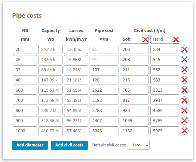
Figure 19: The pipe costs table
Each row in the pipe costs table describes the cost of installing a length of flow and return pipe of a given diameter (Nominal Bore). When the model chooses to install a pipe, it will select the first row from this table whose capacity exceeds the diversified peak capacity that pipe needs to carry.
The columns are:
- NB
- The nominal bore diameter of flow or return in mm. You can add more diameters (rows) using the Add diameter button below.
- Capacity
- The power that can be transmitted by a flow/return pair of this nominal bore. If you don't fill this in, the cell will show THERMOS' estimate, which is controlled by the capacity & loss model below.
- Losses
- The heat losses THERMOS estimates for a flow/return pair per meter. Again, you can enter your own values here, or use the computed values THERMOS estimates.
- Pipe cost
- The cost of the pipe itself, per metre flow/return pair. This is the minimum cost that the model will pay for pipework.
- Civil cost
To the right are multiple civil cost columns. These cover the cost of digging a hole for pipework to go in, for a given diameter, depending on the surface or any other local factors.
You can add more of these with the Add civil costs button below, and you can set which civil costs pertain for paths in the candidate editor. Any path for which civil costs are not selected by hand will take the default civil costs set below the table.
Civil cost names are editable in the table header.
To delete a row click the red cross to its right. To delete a civil cost column, click the red cross by its name.
5.2. Capacity & loss model
The capacity and loss model controls affect how the capacity and losses columns in the table above are calculated. There is more detail about this in the technical description of the model.
You can see the effect by changing the parameters and seeing what happens in the pipe cost table above. Note that changing the medium or flow / return temperature does not affect the cost of supply or cost of heat exchangers, so you must consider these effects yourself.
5.3. Connection costs
Connection costs are intended for covering the cost of equipment within the building, like heat exchangers.
After defining a connection cost here, you can use the candidate editor to assign it to some buildings.
This will determine an extra capital cost, incurred by the network operator in network NPV mode, or by the system in whole-system mode.
5.4. Pumping costs
THERMOS' pumping costs model is simple: pumping overheads are a fixed share of the kWh output from the system, which may have a different price and emissions factor (since they are produced electrically).
In a heat network, pumping overheads offset some heat output from the plant, since the waste heat produced is still useful. In a cold network the opposite is true, and pumping overheads are added to the output needed from the plant.
6. Insulation
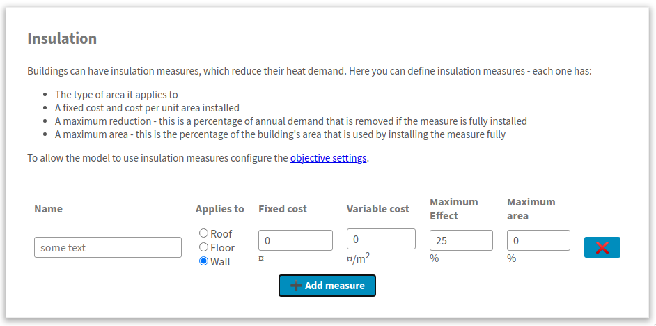
Figure 20: The insulation definitions. Each row defines a type of insulation.
To use insulation you must first put the model into in whole-system mode and enable insulation.
Then you can add some types of insulation using the Add measure button. For each type of insulation you will have to say:
- Name
- this is just descriptive text
- Applies to
- this is the surface the insulation applies to. THERMOS estimates the available area for insulation using the building's footprint, height, and exposed perimeter. The roof and floor areas are taken from the footprint, and the wall area from the exposed (i.e. not touching another building) perimeter multiplied with the height.
- Fixed cost
- this capital cost will be spent if any of this insulation is installed on a building
- Variable cost
- this capital cost is spent per unit area insulated, in addition to the fixed cost
- Maximum effect
- this parameter determines by how much the insulation can reduce overall demand. For example, if maximum effect is 15%, and a building has 200m2 of insulatable area and 5MWh/yr of heat demand, installing all 200m2 will reduce heat demand by 5×0.15 = 0.75 MWh/yr. The model can choose to install any amount between 0 and 200m2, with the effect being pro-rata.
- Maximum area
- this determines the maximum insulatable area as a percentage of the overall area (described above under Applies to). This is to represent things like windows and doors in walls, which would not be covered by insulation.
Finally you will need to mark some buildings as eligible for insulation using the candidate editor (described above).
Insulation definitions can be deleted by clicking the red X button on their row.
7. Individual systems
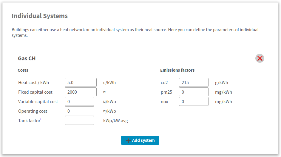
Figure 21: Definitions for an individual system. More can be added by clicking Add system.
To use individual systems you must first put the model into in whole-system mode and enable their use (the checkbox is called "Offer other heating systems" on the objective page).
In network NPV mode, the model will only use individual system definitions when computing the rate for the market tariff.
Then you can add some types of individual systems using the Add system button. For each type of system you will have to say:
- A name
- This is editable by clicking the heading; in the image above clicking "Gas CH" would let you edit the name.
- Heat cost
- This is the cost per kWh delivered heat. If you have a fuel price you need to divide it by system efficiency to get this value.
- Fixed capex
- If this system is installed in a building, this capital cost must be paid.
- Variable capex
- If this system is installed in a building, this capacity-related capital cost is paid per kW of peak demand in the building.
- Tank factor
THERMOS' default peak demand estimates include hot water demand, which makes up most of the peak. This is because heat networks typically provide hot water direct through the heat exchanger, rather than by charging a storage tank.
However, some individual systems do use a hot water tank, and so require a lower peak output. This is represented in THERMOS by the 'tank factor', which is a multiple of the base heat output.
For example, say a building uses 20MWh/yr of heat. Changing the units for this to kW you get about 2.3 kW as the minimum possible peak value (if it were uniformly spread out).
With tank factor set to 1, the peak would be 2.3kW; with tank factor set to 2, it would be 4.6 kW, and so on.
A realistic value for a domestic building is probably in the region of 6.
- Emissions factors
These factors determine the emissions per unit heat produced by the individual system; like the heat cost, you will need to roll any conversion efficiency from fuel into these factors yourself.
They will affect the system cost if there are any emissions prices or limits in effect.
System definitions can be deleted by clicking the red X button to the right of the name.
8. Solution summary
This section only appears after a network problem has run through the optimiser.
It quantitatively describes the solution, without any spatial component.
8.1. Display options
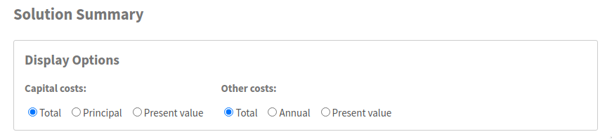
Figure 22: Solution summary display options controls
The display options at the top of the solution summary page control how financial information is rendered in the tables below. The options mean:
- Total
The total un-discounted amount of money spent over the accounting period. This includes all recurring capital costs for replacement equipment, interest payments on annualized capital costs, and all annual operating costs and revenues.
These values are shown in table headers with (¤) as the unit.
- Present value
The discounted version of the total cost; all present and future costs and revenues, discounted and summed.
These values are shown in table headers with (¤PV) as the unit
- Principal
(only shown for capital costs) shows just the principal for a single purchase of the item or items, ignoring repeat payments or interest payments on an annualized cost
These values are shown in table headers with (¤0) as the unit.
- Annual
(only shown for non-capital costs) shows the annual cost or revenue for all costs where this makes sense.
These values are shown in table headers with (¤/yr) as the unit.
Below the display options are a series of subsections and sub-subsections which can be selected by clicking on them:
8.2. Cost summary
The cost summary gives the headline information the model is working on:
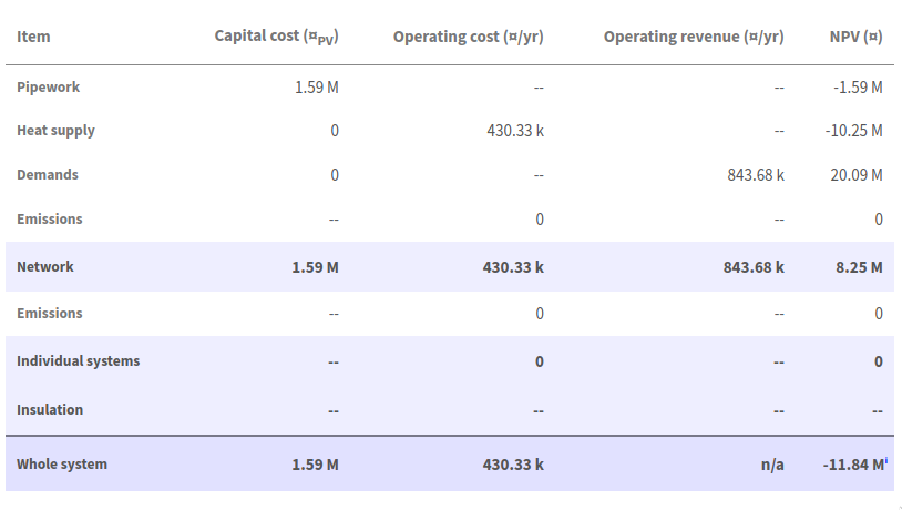
Figure 23: An example of the cost summary table
The two most important figures in the cost summary table are the Network NPV (in the middle on the right) and the Whole system NPV (at the bottom right).
These are the values the model will try and maximize, depending on the choice of objective setting.
The whole system NPV will always be negative, because the model only displays costs - the benefit is in terms of delivered heat, which is assumed to be a non-negotiable good desirable at any price.
8.3. Network (Pipework)
The pipework section of the network tab lists all the pipe used in the network, broken down by civil cost category and installed diameter.
For more detailed breakdowns you will want to download the results in a spreadsheet and analyse them outside the application.
8.4. Network (Demands)
The demands section lists all demands connected to the network, and shows the cost and revenue associated with them. If they have user-defined fields, you can group them by these fields with the menu in the top left of the table.
8.5. Network (Supplies)
The supplies section describes each supply point in the network; the columns are:
- Capacity
- This is the size of plant needed to meet the diversified peak load
- Output
- This is the heat output needed from the plant, including losses. In heat network mode this is net of pumping energy, in cold network mode it will include pumping energy.
- Pumping
- The power required for pumping (see above for how to set pumping costs).
- Capital
- The capital cost for the plant (units determined by display options above)
- Capacity
- The operating cost related to plant capacity
- Heat
- The operating cost related to production of heat (in the output column)
- Pumping
- The operating cost from pumping energy
- Coincidence
- The coincidence factor applied to the peak loads this plant is serving.
8.6. Individual systems
If the model has installed any individual systems (see above for individual system definitions), this will list the buildings which got them, and their costs.
8.7. Insulation
If the model has installed any insulation on buildings this section lists the quantity, cost and effect of insulation installed.
8.8. Emissions
This gives a breakdown of the emissions in the solution by cause, in terms of their quantities and their costs. Costs are affected by the emissions cost settings in the objective page.
8.9. Optimisation
This page shows some technical information about the optimisation itself. The values displayed are:
- Objective value
- This is the objective value as seen by the optimiser after correcting the diversity and heat loss parameters, but without rounding up pipe diameters.
- Runtime
- The time spent in the optimiser
- Iterations
- The number of mixed-integer programs solved
- Iteration range
- The range in objective value encountered while iterating to find good parameters.
- Gap
- The MIP gap; this is an upper bound on how close the optimiser is to finding the best possible solution; if zero, the solution is optimal. However, this number is confounded by the effect of parameter fixing. The value shown is the gap for the solution based on estimated parameters.
- Bounds
- These are the bounds on the optimum value of the best solution found, again confounded by parameter estimation. The true optimum is probably somewhere in this range. Note that the objective value shown above may lie outside this range because it is the value for a slightly different problem in which the parameters have been re-estimated.
9. Run log
The run log is displayed when there is a solution; it contains some diagnostic text output from the optimisation model. The text is not guaranteed to stay the same or to mean anything useful.
10. Importing and exporting data
Near the bottom of the sidebar is a section titled Import / Export Data, under which are three links:
- ↓ Excel spreadsheet
- This link will download the information shown in the editor as an excel spreadsheet.
- ↑ Excel spreadsheet
- This link will ask you to upload an excel spreadsheet, in the same form as the previous link downloads. Some data from the uploaded spreadsheet will be loaded into the problem, detailed below.
- ↓ Geojson
- This link will download a GIS representation of the problem, which contains the information you can see on the map.
10.1. Uploadable parameters
Only information from these sheets in the output spreadsheet will be loaded when you import it by uploading:
- Tariffs
- Connection costs
- Individual systems
- Pipe costs
- Insulation
- Other parameters
- Capital costs
- Supply plant
- Supply profiles
- Supply storage
- Supply parameters
These all contain parameters that control the model, but no information about specific buildings or roads.
When you upload a spreadsheet the application will show a dialog asking what parameters you want to use and two other questions:
- Whether to use new parameters where names match
- Whether to keep old parameters with different names
These settings control how existing relationships between buildings and parameters are affected by an upload.
For example, if you have some paths with a civil cost of "Hard Dig" in your problem and you upload a spreadsheet and select to use the pipe costs data, the possible outcomes are:
- If the uploaded spreadsheet contains a civil cost called "Hard Dig" as well:
- If you have selected to new parameters where names match
- The paths that previously used "Hard Dig" will now use the new civil cost called "Hard Dig"
- If you have selected not to use new parameters where names match
- Existing assignments to "Hard Dig" will be cleared
- If you have selected to new parameters where names match
- If the spreadsheet does not contain "Hard Dig"
- If you have selected to keep parameters with different names
- The existing paths will be unaffected
- If you have selected not to keep parameters with different names
- The "Hard Dig" civil cost will be removed entirely from the problem
- If you have selected to keep parameters with different names
11. Concepts
11.1. Constraint status
THERMOS is an optimising model which means it makes some decisions.
The main decision is whether to put something in a heat network.
The constraint status of an item affects whether the optimiser can or must use it in a network.
- If the status is forbidden, the item is ignored
- If the status is optional, the item will be included in a network if that is an improvement on any alternative
- If the status is required, the item must be connected to a network if at all possible
11.2. Tariffs
THERMOS uses tariffs when it is in network NPV mode to decide how much revenue the network will get from a customer.
11.3. Market tariff
The market tariff is a special tariff THERMOS uses, in which a unit rate for heat is chosen that is a bit better than the next best alternative for the building.
11.4. Civil costs
Civil engineering costs are one of the costs associated with installing a pipe.
They are to do with digging a hole and filling it back in and making good, so they are affected by the surface being dug, the location of the dig and so on.
They don't include the cost that is the same anywhere in a city: this is the cost of the pipe and mechanical engineering (welding etc) required to fit the pipe.
11.5. Connection costs
Connection costs represent the cost of all the equipment required within a building to connect it to a heat network.
Typically this would be a heat exchanger, and maybe some internal pipework.
11.6. Annual and peak demand
THERMOS' network model considers only two types of demand:
- The annual demand in kWh/yr
- The peak demand in kW
This is because, by and large, a network connection's size is determined by peak demand, and its operations are determined by annual demand.
11.7. Tank factor
THERMOS includes an invented quantity called the "Tank factor".
This exists to reflect the fact that whilst heat network connections are usually sized for hot water production on demand, other heating systems are not. Heat pumps, for example, would have to be very large to deliver the ~20-30 kW of heat needed for instant hot water.
These systems are instead installed with a hot water tank which acts as storage.
The tank factor is used to adjust the peak demand for these systems, by expressing it as a multiple of the minimum possible peak demand (i.e. the annual demand expressed in kW).
11.8. Pipe heat loss
Heat network pipes lose heat into the the ground, because they are warmer than the ground.
In THERMOS you can either enter your own losses per metre, or use the built-in model.
If you use the built-in model you probably want to set the ground temperature. If this is higher, the heat losses will be reduced.
11.9. Diversity / coincidence
Load diversity and coincidence are two sides of the same coin.
As mentioned above, heat networks are usually sized for hot water.
When there are several buildings connected to a network, it is not often a requirement for them all to have hot water on demand at the same time, because hot water usage is a bit stochastic (moreso than heat usage).
Diversity or coincidence is a factor used to approximate this effect.
For example if two buildings have a peak demand of 30kW, we might only supply them using a shared pipe with capacity to deliver 48kW, which is not 30kW + 30kW. This would be a coincidence of 80% - we only size for 80% of the shared demand.
11.10. Objective
The objective is the technical term for a number that the model is trying to make as large as possible.
For THERMOS this number is always the present value (or minus the present cost).
In network NPV mode it is the present value to the network operator of their revenues less their costs.
In whole-system mode it is minus the present cost of all the costs of delivering the heat.