The THERMOS supply model is accessed through the same user interface as the network model.
You should read the section on the network model user interface first.
To run the supply model you must first have defined and solved a THERMOS network problem. This is because the demand profile that the supply model must meet is defined by the buildings that have been connected to the network. More details of this are in the section describing the relationship between network and supply models.
To understand the meaning of the day types and intervals described below you may also want to read the relevant section in the technical description before continuing.
1. Running the supply model
To run the supply model, click the Optimise button in the top right corner, and select either Supply or Both.
Because the supply model is quite fast compared to the network model, once you have a network solution it will be much quicker to reevaluate your supply solution by clicking only Optimise → Supply
2. Supply model parameters
Apart from the connection to the network model, all supply parameters are found in the application sidebar under Supply Problem.
2.1. Profiles
The profiles section is all about how the supply model represents time.
A representative year of operation is broken down into a number of characteristic day types, which are each broken down into a number of intervals. In each of these intervals the supply model can consider different heat demand, fuel prices, emissions factors and so on.
Every building that is being considered by the supply model has an associated heat profile, which says when in the representative year the building's demand occurs.
Heat profiles for all connected buildings are combined together to produce a single overall profile, which is the demand that the supply must serve.
2.1.1. Default profile
This lets you set which profile buildings should have, if you have not set a profile.
The network model help describes how to select what profiles individual buildings have, if you don't want them to take this default.
2.1.2. Day types
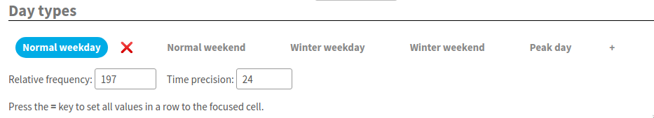
Figure 1: Setting up supply day types.
At the top of the day types section is a row which contains the names of the day types. In the picture above you can see labels for the five default day types: normal weekday, normal weekend, winter weekday, winter weekend and peak day.
Clicking on these labels switches which day type is displayed in the rest of the page. The selected day type is shown in blue.
You can delete the selected day type by clicking the red cross next to the name, and you can rename it by clicking the name, typing in a new name, and pressing the enter key.
You can add an entirely new day type by clicking the + on the right hand end, typing in a name for the new day type, and pressing the enter key.
Below the list of day types are two fields that let you change how important the day type is, and how it is divided up:
- Relative frequency
- This controls how many days per year the selected day type represents. The frequency here is relative to the summed relative frequency of all the day types, which could add up to more than 365.
- Time precision
- This controls how many intervals the day is split up into. Each interval has a column in the rest of the page. For example, if time precision is 24, each cell represents one hour of the day. If it is 12, each cell represents a two-hour period, and so on.
2.1.3. Heat profiles
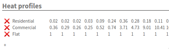
Figure 2: Supply heat profiles section showing some of the default profiles.
Each row in the heat profiles section effectively defines a type of building for the supply model. In the image above there are three types displayed, Residential, Commercial and Flat.
New heat profiles can be added by clicking the + at the bottom, entering a name, and pressing the enter key. Existing ones can be deleted with the X to the left of their name.
The name itself and the values to the right can be changed by clicking and typing, as usual.
The values to the right require a little explanation:
- Each column of values describes a given time interval in the currently selected day type
- The values in the row are dimensionless; they are all relative to the maximum value for that heat profile across all day types. To understand how the values are used you should read the section on how the network and supply model are connected.
2.1.4. Fuels
Below the heat profiles are the fuels' prices and emissions.
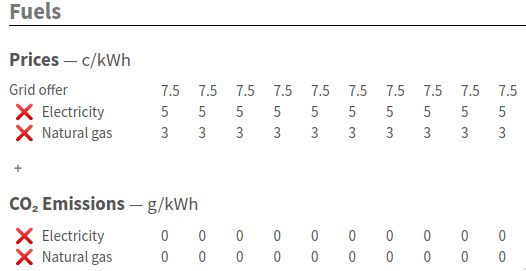
Figure 3: Some of the supply fuels section
At the top you can set the fuels prices within each time interval in the current day type. There is a special row in this section called Grid offer which reflects the electricity price at which the grid will buy CHP output in this time interval - see below under supply technologies for how to designate CHP.
If you want to add or remove a fuel use the + and ❌ buttons respectively.
Below fuel prices you can also enter emissions factors for a fuel.
As a convenience, if you want to set an emissions factor the same for all the intervals in a day type, put the value you want in a particular cell and then press =, which will copy that value for the other intervals in that day.
This key also works in all the other rows, but it is most likely to be useful here.
2.1.5. Substation load
Each row in the substation load section describes the pre-existing load on one of the substations defined in the technologies page (described below) in MW substation output. This affects the headroom at the substation in that interval.
2.2. Technologies
The technologies page contains three sections, for each of the system components that the supply model considers:
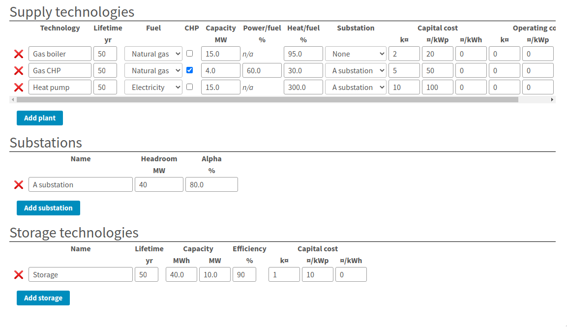
Figure 4: Supply technologies page
2.2.1. Supply technologies
The first section gives the plant types.
Each row in this table defines an option that the supply model can decide to purchase or not to purchase in order to meet the demand for heat. If a particular technology is used in any time interval it must be paid for.
The columsn in the table mean:
- Technology
- This is a descriptive name for the technology, for display purposes. It doesn't mean anything to the computer
- Lifetime
- This is how long the plant lasts before it must be replaced. This is connected to the accounting period in the objective page; the number of times the capital cost will be paid is determined by the ratio of lifetime to accounting period.
- Fuel
This menu lets you choose one of the fuels defined on the fuels section of the profiles page. This relationship will determine the cost of producing heat and the associated emissions.
Note that the name of the fuel is not meaningful to the computer; special behaviour about electricity is determined by the CHP and substation columns alone, so you can say that the fuel is "Natural gas" but still have a substation and use up its headroom!
- CHP
- If checked, the plant is a CHP engine. In this case as well as incurring cost for consuming fuel, the plant can produce revenue by selling fuel at the grid offer price.
- Capacity
- This is the maximum rate of output this type of plant can produce in any given time interval.
- Power / fuel
This cell is only relevant when the CHP box is ticked. It gives the electrical generating efficiency of the CHP, in terms of electricity produced per unit fuel consumed.
If the objective section has heat dumping allowed then the model will allow the CHP to be power led, if that produces a better NPV. Otherwise, the CHP will only produce electricity as a side-effect of a decision to produce heat.
- Heat / fuel
- This determines the amount of heat the plant can produce for the network per unit of fuel consumed.
- Substation
This menu lets you select a substation to connect the plant to; substations constrain plant operations beyond the capacity column as they may have limited headroom and can be shared between plant.
If a plant is not marked as CHP then it is assumed to draw power from the substation, using up some of the substation's headroom.
Conversely, CHP plant is assumed to put power into the substation, possibly increasing its headroom or potentially using it up in the other direction (as "reactive power")
- Capital cost
- The capital cost terms affect the cost of purchasing the plant, in three parts
- k¤
- A fixed cost in thousands of currency
- ¤/kWp
- A cost per unit capacity, which is multiplied with the maximum power output in any interval of the plants operation.
- ¤/kWh
- A cost per unit output, which is multiplied with the total annual output of a typical year to give a one-off capital cost.
- Operating cost
- The operating cost terms are used to produce an annual operating cost which is incurred every year in the accounting period.
- k¤
- A fixed annual cost in thousands of currency.
- ¤/kWp
- A variable annual cost multiplied with the peak output.
- ¤/kWh
- A variable annual cost multiplied with the total annual output.
2.2.2. Substations
A substation represents a limited connection to the electrical grid. Each substation has only 3 parameters:
- Name
- This is displayed in the substation column of the table above, and as the row label for the substation load section of the profiles page.
- Headroom
- This gives the maximum electrical power the substation can deliver to all its connected loads before it melts.
- Alpha
This determines the headroom in the reverse direction. For example, a substation with 40MW headroom and an alpha of 80% can deliver 40MW from HV to LV ("grid" to "consumer"), but it can only take 32MW of power input from LV and send it back to HV.
This is relevant to CHP systems, where it will limit how much power they can output.
In every time interval, the total power output from a substation must be between (Headroom - Existing Substation Load) and (-Headroom × Alpha). This limits the power that can be drawn or sent to the substation to lie in this range.
2.2.3. Storage technologies
Heat storage technologies are another component the plant can buy. The model only understands within-day storage at the moment.
Each row in the storage technologies table represents a type of storage the model can buy. If the model buys some storage, it can then choose to charge it during one time interval and discharge it during a later interval on the same day.
This lets the model use fuel when it is cheap to deliver heat when fuel would be expensive, and to reduce the size of plant it must purchase.
The storage parameters are:
- Name
- A descriptive name for the technology
- Lifetime
- The lifetime of the technology in years; this affects how often the capital cost must be paid.
- Capacity (MWh)
- This gives the maximum size of store that can be purchased, in terms of how much charge it can hold.
- Capacity (MW)
- This gives the maximum rate at which the store can be charged or discharged
- Efficiency
- This determines how much heat must be put in to get a unit of heat out.
- Capital cost
- Determines how much needs to be paid each time the lifetime expires.
- k¤
- A fixed annual cost in thousands of currency.
- ¤/kWp
- A variable annual cost multiplied with the peak output from the store.
- ¤/kWh
- A variable annual cost multiplied with the maximum charge in the store.
2.3. Objective
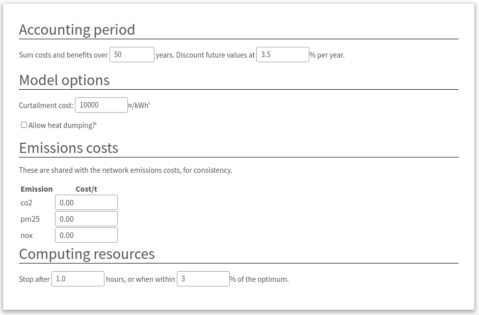
Figure 5: Supply objective parameters
The supply objective page controls some parts of the optimisation for the supply model:
- Accounting period
- These settings affect how capital and operating costs are combined across time into a single value. Repeating costs are extended over the given number of years, and discounted using conventional geometric discount rate each year.
- Curtailment cost
The curtailment cost is a synthetic cost for the price of undersupplying heat. This makes sure that the model can always find a solution, rather than becoming infeasible if there is insufficient capacity at some point in time.
By looking in the results for curtailment you can see when there is not enough capacity and adjust the problem.
The default value for this is probably fine, but you could increase it if you found that the model was choosing curtailment because the alternative was feasible but exceedingly expensive.
- Allow heat dumping
- If ticked this will allow CHP supplies to be power-led rather than heat-led, so they may produce more than the demand for heat if the sales price of electricity justifies it.
- Emissions costs
- These values determine the operating cost incurred by producing emissions. Editing the costs on this page will also edit them on the network model's optimisation settings page, and vice-versa
- Computing resources
- The computing resources settings control how long the supply model can run for. It usually runs very fast and finds an exact answer, so you are unlikely to need to adjust these.
3. Supply solution
The supply solution page is broken into sections which you can hide or show by clicking on their headings:
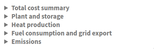
Figure 6: Supply solution headings. Clicking on one of the headings will rotate the triangle and show some more information.
3.1. Total cost summary
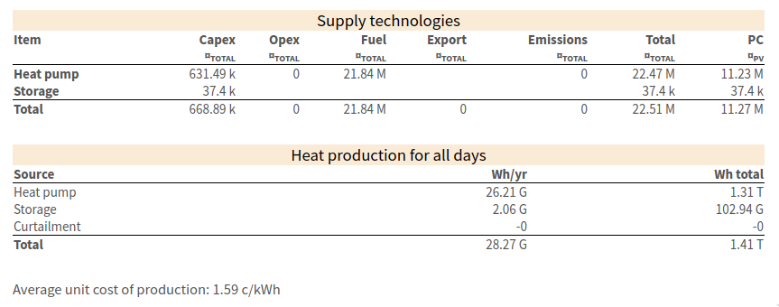
Figure 7: The total cost summary section showing headline results for the supply model
The total cost summary section describes the costs and output of the system. The top table describes the cost of what was built - all columns except the rightmost give the undiscounted total financial value for the column. Each row above the total line describes a part of the system that was built.
The bottom table shows total heat production per year and over the accounting period. The curtailment row is special - if it is nonzero then the model has decided it is cheaper to undersupply heat according to the curtailment cost setting, or impossible to avoid doing this.
The average unit cost shown at the bottom simply divides the total heat output by the total cost for all time (so it is not discounted).
3.2. Plant and storage
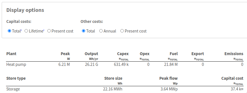
Figure 8: The plant and storage section, showing details of the technologies purchased.
At the top of this section are some controls which let you change the financial units in the columns below. These are analogous to the similar controls in the network solution summary.
Below that are two tables, one describing all the heat plant built, and one all the storage built. For each plant row you can see the peak and annual output for that plant, and for store rows the size and the peak flow. These values determine the capital and operating costs for the technologies which are set up in the supply technologies section.
3.3. Heat production
The heat production section shows two types of information - a series of bar charts which show how the system is making its required output on each day type in each interval, and then a series of summary tables for each day type describing the peak and total output.
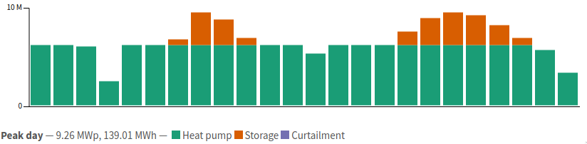
Figure 9: A single graph from the heat production section. The bars give the power output from storage and supply technologies in each time interval of a day. The caption at the bottom describes the dimensions of the graph. In this case, it is for the "Peak day" day type. Next to that you can see the peak output and then the area under the graph (for a single day of this type). In this case you can see the heat pump runs nearly continuously, with the absolute peak being made up by storage.
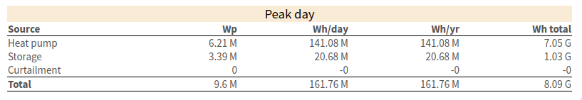
Figure 10: The corresponding table for the peak day. The table's header line gives the day type, and the rows the peak and total production of heat on that day. The columns to the right show how much this day type contributes to the year and to the whole accounting period.
3.4. Fuel consumption and grid export
The fuel consumption and grid export section is very similar to the heat production section. However, instead of showing heat output by system, the graphs and tables show fuel input by type of fuel.
3.5. Emissions
The emissions section displays an overall summary table for annual or lifetime emissions from the system, giving their amount and cost.
4. Downloading results and parameters
The results and parameters for the supply model can be downloaded in the same way as those for the network model. Click the THERMOS logo in the top left to open the sidebar, and then choose ↓ Excel Spreadsheet under the Import/Export Data heading.
This will give you a spreadsheet in which the following pages are about the supply:
- Supply Plant
- Contains the plant parameters from the supply technologies page
- Supply Storage
- Contains the storage parameters from the supply technologies page
- Supply day types
- Contains the definitions of each day type from the profiles page
- Supply profiles
- Contains the input profiles for each day type from the profiles page
- Supply operations
- (present if there is a solution) Contains the operational decisions from the supply model, in terms of how much output each component makes in each time interval
5. Uploading parameters
All of the supply parameters above will be loaded in if you upload a spreadsheet via the sidebar's ↑ Excel Spreadsheet option, so you can edit profiles and other datasets this way.
The easiest option here is to download a spreadsheet, edit it, and then load it back in.